머신러닝 수업 2주차
Regularization
Ridge Regularization
- Applies to both over and under determined systems.
- The loss function of the ridge regression is defined as the loss function
- $|\theta|^2$ : Regularization function
- $\lambda$ : Regularization parameter
- The solution of the ridge regression is
which gives us $\hat{\theta}=(A^{\top}A+\lambda I)^{-1}A^{\top}{\bf{y}}$
Change in Eigen-values
Ridge regression improves the eigen-Values
- Eigen-decomposition of $A^{\top}A$:
where $U=$ eigen-value matrix, $S=$ eigen-value matrix.
-
$S$ is a diagonal matrix with non-negative entries:
-
Therefore, $S+\lambda I$ is always positive for any $\lambda > 0$, implying that
- If $\lambda \rightarrow 0$, then $\hat{\theta}=(A^{\top}A)^{-1}A^{\top}{\bf{y}}$
- If $\lambda \rightarrow \infty$,
- There is a trade-off curve between the two terms by varying $\lambda$.
Comparing Vanilla and Ridge
Suppose ${\bf{y}}=A\theta^* + {\bf{e}}$ for some ground truth $\theta^*$ and noise vector ${\bf{e}}$. Then, the vanilla linear regression will give us
\[\hat{\theta}=(A^\top A)^{-1}A^\top {\bf{y}}\] \[=(A^\top A)^{-1}A^\top (A\theta^*+{\bf{e}})\] \[=\theta^*+(A^\top A)^{-1}A^{\top}{\bf{e}}\]If ${\bf{e}}$ has zero mean and varianze $\sigma^2$, we can show that
\[\mathbb{E}[\hat{\theta}]=\theta^*\] \[\text{Cov}[\hat{\theta}]=\sigma^2(A^\top A)^{-1}\]Therefore, the regression coefficients are unbiased but have large variance. We can further show that the mean-squred error(MSE) is
\[\text{MSE}(\hat{\theta})=\sigma^2\text{Tr}\{ (A^\top A)^{-1} \}.\]On the other hand, if we use ridge regression, then
\[\hat{\theta}(\lambda)=(A^\top A + \lambda I)^{-1}A^\top (A\theta^*+{\bf{e}})\] \[=(A^\top A + \lambda I)^{-1}A^{\top}A\theta^*+(A^\top A + \lambda I)^{-1}A^\top{\bf{e}}\]Again, if ${\bf{e}}$ is zero mean and has a variance $\sigma^2$, then
\[\mathbb{E}[\hat{\theta}(\lambda)]=(A^\top A+\lambda I )^{-1}A^\top \theta^*\] \[\text{Cov}[\hat{\theta}(\lambda)]=\sigma^2(A^\top A + \lambda I)^{-1}A^\top A(A^\top A+\lambda I)^{-\top}\] \[\text{MSE}[\hat{\theta}(\lambda)]=\sigma^2\text{Tr}\{ W_\lambda(A^\top A)^{-1}W^\top_\lambda \}+\theta^{*\top}(W_\lambda - I)^\top(W_\lambda -I)\theta^*\]where $W_\lambda=(A^\top A + \lambda I)^{-1}A^\top A$. In particular, we show that
Theorem(Theobald 1974)
For $\lambda < 2\sigma^2|\theta^*|^{-2}$, it holds that $\text{MSE}(\hat{\theta}(\lambda)) < \text{MSE}(\hat{\theta})$
Choosing $\lambda$
Because the following three problems are equivalent
\[\theta^{*}_\lambda=\text{argmin}_\theta\|A\theta-{\bf{y}}\|^2+\lambda\|\theta\|^2\]subject to $|\theta|^2\leq\alpha$
\[\theta^{*}_\alpha=\text{argmin}_\theta\|A\theta-{\bf{y}}\|^2\]subject to $|A\theta-{\bf{y}}|^2 \leq \epsilon$
We can seek $\lambda$ that satisfies $|\theta|^2 \leq \alpha$ :
- You know how much $|\theta|^2$ would be appropriate.
We can seek $\lambda$ that satisfies $|A\theta -{\bf{y}}|^2 \leq \epsilon$
- You know how much $|A\theta-{\bf{y}}|^2$ would be tolerable.
Other approaches:
- Akaike’s information criterion: Balance model fit with complexity
- Cross validation: Leave one out
- Generalized cross-validation: Cross-validation + weight
LASSO Regression
-
An alternative to the Ridge Regression is Least Absolute Shrinkage and Selection Operator (LASSO)
-
The loss function is
- Intuition behind LASSO: Many features are not active.
Interpreting the LASSO Solution
\[\hat{\theta}=\text{argmin}_\theta\|A\theta-{\bf{y}}\|^2+\lambda\|\theta\|_1\]- $|\theta|_1$ promotes sparsity of $\theta$. It is the nearest convex approximation to $|\theta|_0$, which is the number of non-zero.
Why are Sparse Models Useful?
-
Images are sparse in transform domains, e.g., Fourier and wavelet.
-
Intuition: There are more low frequency components and less high frequency components
-
Examples above: $A$ is the wavelet basis matrix. $\theta$ are the wavelet coefficents.
-
We can truncate the wavelet coefficients and retain a good image.jpg
-
Many image comression schemes are based on this, JPEG, JPEG2000.
LASSO for Image Reconstruction
Image inpainting via KSVD dictionary-learning
-
$y=$ image with missing pixels. $A=$ a matrix storing a set of trained feature vectors (called dictionary atoms). $\theta=$ coefficients.
-
minimize $|{\bf{y}}-A\theta|^2+\lambda|\theta|_1$
-
KSVD = k-means + Singular Value Decomposition (SVD) : A method to train the feature vectors that demonstrate sparse representations.
Shrinkage Operator
The LASSO problem can be solved using a shrinkage operator. Consider a simplified problem (with $A=I$)
\[J(\theta)={1 \over 2} \|{\bf{y}}-\theta\|^2+\lambda\|\theta\|_1\] \[=\sum^d_{j=1} ({1 \over 2}(y_j-\theta_j)^2+\lambda\|\theta_j\|_1 )\]Since the loss is separable, the optimization is solved when each individual term is minimized. The individual problem
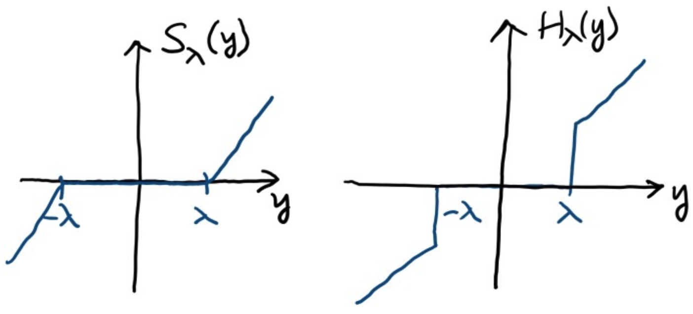
\[\hat{\theta}=\text{argmin} \{ {1 \over 2}(y-\theta)^2+\lambda|\theta| \}\] \[=\text{max}(|y|-\lambda, 0)\text{sign}(y)\] \[=S_\lambda(y)\]Shrinkage VS Hard Threshold
-
The shrinkage operator looks as follows.
-
Any number between $[-\lambda, \lambda]$ is “shrink” to zero.
-
Try compare with the hard threshold operator $H_\lambda(y)=y\cdot { |y|\geq \lambda }$
Algorithms to Solve LASSO Regression
In general, the LASSO problem requires iterative algorithms:
ISTA Algorithm (Daubechies et al. 2004)
- For $k=1,2,…,$
- $v^k=\theta^k-2\gamma A^\top(A\theta^k-{\bf{y}})$
- $\theta^{k+1}=\text{max}(|v^k|-\lambda, 0)\text{sign}(v^k)$
FISTA Algorithm (Beck-Teboulle 2008)
- For $k=1,2,…,$
- $v^k=\theta^k-2\gamma A^\top(A\theta^k-{\bf{y}})$
- $z^k=\text{max}(|v^k|-\lambda, 0)\text{sign}(v^k)$
- $\theta^{k+1}=\alpha_k\theta^k+(1-\alpha_k)z^k$
ADMM Algorithm (Eckstein-Bertsekas 1992, Boyd et al. 2011)
- For $k=1,2,…,$
- $\theta^{k+1}=(A^\top A+\rho I)^{-1}(A^{\top}y+\rho z^k-u^k)$
- $z^{k+1}=\text{max}(|\theta^{k+1}+u^k\rho|-\lambda / \rho, 0) \text{sign}(\theta^{k+1}+u^k/\rho)$
- $u^{k+1}=u^k+\rho(\theta^{k+1}-z^{k+1})$
And many others.
Example: Crime Rate Data
| city | funding | not-hs | college | college4 | crime rate |
|---|---|---|---|---|---|
| 1 | 40 | 74 | 11 | 20 | 478 |
| 2 | 32 | 72 | 11 | 18 | 494 |
| 3 | 57 | 70 | 18 | 16 | 643 |
| 4 | 31 | 71 | 11 | 19 | 341 |
| 5 | 67 | 72 | 9 | 24 | 773 |
| … | … | … | … | … | |
| 50 | 66 | 67 | 26 | 16 | 940 |
Consider the following two optimizations
\[\hat{\theta}_1=\text{argmin}_\theta J_1(\theta)=\|A\theta-{\bf{y}}\|^2+\lambda \|\theta\|_1\] \[\hat{\theta}_2=\text{argmin}_\theta J_2(\theta)=\|A\theta-{\bf{y}}\|^2+\lambda \|\theta\|_2\]Comparison between L-1 and L-2 norm
-
Plot $\hat{\theta}_1(\lambda)$ and $\hat{\theta}_2(\lambda)$ vs. $\lambda$.
- LASSO tells us which factor appears first.
- If we are allowed to use only one feature, then % high is the one.
- Two features, then % high + funding.
Pros and Cons
Ridge regression
- (+) Analytic solution, because the loss function is differentiable.
- (+) As such, a lot of well-established theoretical gurantees.
- (+) Algorithm is simple, just one equation.
- (-) Limited interpretability, since the solution is usually a dense vector.
- (-) Does not reflect the nature of certain problems, e.g., sparsity
LASSO
- (+) Proben applications in many domains, e.g., images and speechs.
- (+) Echoes particularly well in modern deep learning where parameter space is huge.
- (+) Increasing number of theoretical guarantees for special matrices.
- (+) Algorithms are available.
- (-) No closed-form solution. Algorithms are iterative.
Regularization
Weight Decay
- L2 Regularization (learning rate, gradient, gradient of l2-regularization)
- Penalizes large weights
- Improves generalization
Early stopping
- Easy form of regularization
Bagging and Ensemble Methods
-
Train multiple models and average their results.
-
E.g., use a different algorithm for optimization or change the objective function / loss function.
-
If errors are uncorrelated, the expected combined error will decrease linearly with the ensemble size.
-
Bagging: uses k different datasets.
Dropout
-
Disable a random set of neurons (typically 50%)
- Using half the network = half capacity
- Redundant representations
- Base your scores on more features
- Consider it as a model ensemble.
- Two models in one.
- Training a large ensemble of models, each on different set of data(mini-batch) and with SHARED parameters $\rightarrow$ Reducing co-adaption between neurons
Dropout: Test Time
-
All neurons are “turned on” - no dropout $\rightarrow$ Conditions at train and test time are not the same.
- Test : $z=(\theta_1x_1+\theta_2 x_2) \cdot p$, p is a dropout probability
- Train :
Dropout: Verdict
-
Efficient bagging method with parameter sharing
-
Try it!
-
Dropout reduces the effective capacity of a model $\rightarrow$ larger models, more training time.
Batch Normalization
- Wish: Unit Gaussian activations (in our example)
- Solution: let’s do it
-
All we want is that our activations do not die out
-
In each dimension of the features, you have a unit gaussian (in our example)
-
For NN in general $\rightarrow$ BN normalizes the mean and variance of the inputs to your activation functions
-
A layer to be applied after Fully Conneted layers and before non-linear activation functions.
- Normalize
The network can learn to undo the Normalization
\[r^{k}=\sqrt{Var[x^{(k)}]}\] \[\beta^{(k)}=E[x^{(k)}]\]- Allow the network to change the range
-
OK to treat dimensions separately? Shown empirically that even if features are not correlated, convergence is still faster with this method
-
You can set all biases of the layers before BN to zero, because they will be cancelled out by BN anyway.
BN: Train vs Test
Training : Compute mean and variance from mini-batch 1,2,3…
Testing : Compute mean and variance by running an exponentially weighted averaged across training mini-batches. Use them as $\sigma^2{test}$ and $\mu{test}$
\[Var_{running}=\beta_{m}*Var_{running}+(1-\beta_m)*Var_{minibatch}\] \[\mu_{running}=\beta_{m}*\mu_{running} + (1-\beta_m)*\mu_{minimbatch}\]$\beta_m$ : momentum (hyperparameter)
BN: What do you get?
-
Very deep nets are much easier to train $\rightarrow$ more stable gradients
-
A much larger range of hyperparameters works similariy when using BN
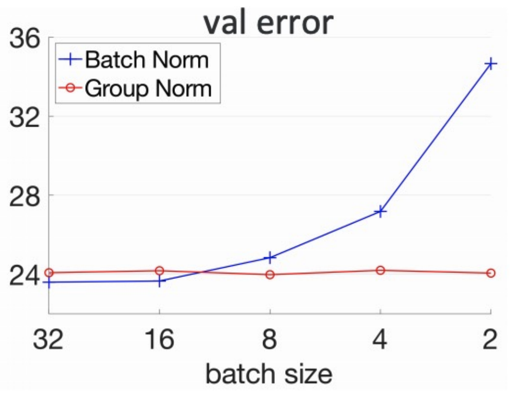
Other Normalizations
Data Augmentation
-
A classifier has to b einvariant to a wide variety of transformations
-
Helping the classifier: synthesize data simulating plausible transformations
Data Augmentation: Brightness
- Random brightness and contrast changes
Data Augmentation: Random Crops
- Training: random crops
- Pick a random L in [256, 480]
- Resize training image, short side L
- Randomly sample crops of 224x224
- Testing: fixed set of crops
- Resize image at N scales
- 10 fixed crops of 224x224:(4corners + 1center) x 2 flips
Data Augmentation
-
When comparing two networks make sure to use the same data augmentation!
-
Consider data augmentation a part of your network design
Kernel Method
Why Another Method?
- Linear regression: Pick a global model, best fit globally.
- Kernel method: Pick a local model, best fit locally.
- In kernel method, instead of picking a line / a quadratic equation, we pick a kernel.
- A kernel is a measure of distance between training samples.
- Kernel method buys us the ability to handle nonlinearity.
- Ordinary regression is based on the columns (features) of A.
- Kernel method is based on the rows (samples) of A.
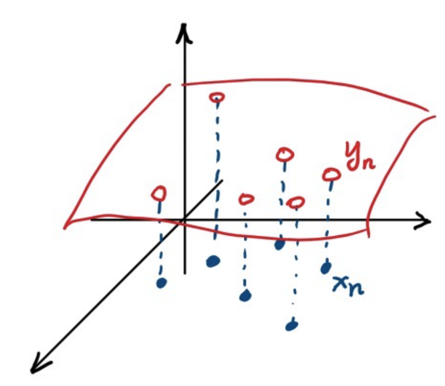
Pictorial Illustration
- goal : learn the surface
- prediction : when new sample comes, interpolate on the surface
Overview of the Method
Model Parameter
- We want the model parameter $\hat{\theta}$ to look like:
- This model expresses $\hat{\theta}$ as a combination of the samples.
- The trainable parameters are $\alpha_n$, where $n=1,…,N$.
- If we can make $\alpha_n$ local, i.e., non-zero for only a few of them, then we can achieve our goal: localized, sample-dependent.
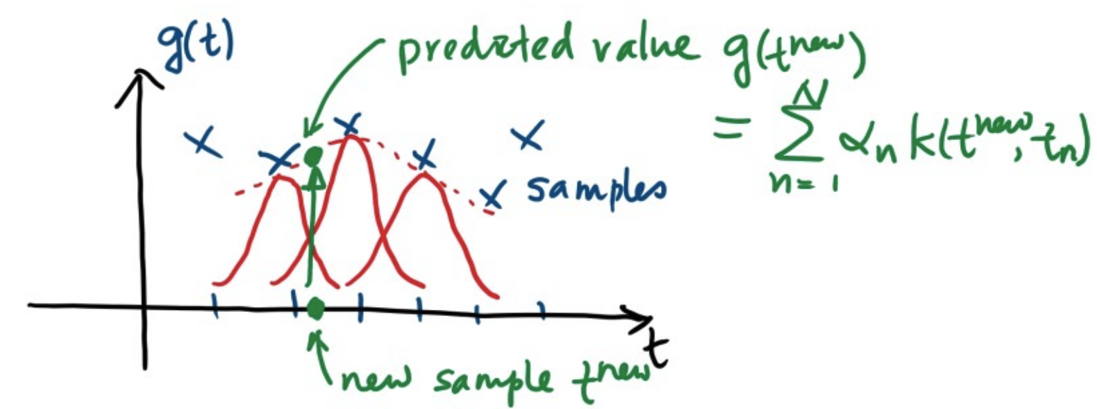
Predicted Value
- The predicted value of a new sample $x$ is
Dual Form of Linear Regression
Goal : Address Question 1: Express $\hat{\theta}$ as
\[\hat{\theta}=\sum^N_{n=1}\alpha_nx^n\]We start by listing out a technical lemma:
Lemma
For any $A \in \mathbb{R}^{N\times d}$, $y\in \mathbb{R}^d$, and $\lambda > 0$
\[(A^{\top}A+\lambda I)^{-1}A^{\top}y=A^\top(AA^{\top}+\lambda I)^{-1}y\]Remark:
- The dimensions of $I$ on the left is $d \times d$, on the right is $N \times N$.
- If $\lambda=0$, then the above is true only when $A$ is invertible.
Dual Form of Linear Regression
- Using the Lemma, we can show that
Primal Form
\[\hat{\theta}=(A^\top A+\lambda I)^{-1}A^{\top}y\]Dual Form
\[\hat{\theta}=A^{\top}(AA^{\top}+\lambda I)^{-1}y\]The solution to the dual problem provides a lower bound to the solution of the primal problem.
\[=\begin{bmatrix} -(x^1)^{\top}- \\ -(x^2)^{\top}- \\ ... \\ -(x^N)^{\top}-\end{bmatrix}^{\top} \begin{bmatrix} \alpha_1 \\ ... \\ \alpha_N \end{bmatrix}=\sum^N_{n=1}\alpha_nx^n\] \[\alpha_n=[(AA^\top+\lambda I)^{-1}y]\]The Kernel Trick
Goal: Addresses Question 2: Introduce nonlinearity to
\[\hat{y}=\hat{\theta}^\top x = \sum^N_{n=1}\alpha\langle x, x^n\rangle\]The Idea:
- Replace the inner product $\langle x, x^n \rangle$ by $k(x, x^n)$:
- $k(\cdot, \cdot)$ is called a kernel.
- A kernel is a measure of the distance between two samples $x^i$ and $x^j$.
- $\langle x^i, x^j \rangle$ measure distance in the ambient space, $k(x^i, x^j)$ measure distance in a transformed space.
- In particular, a valid kernel takes the from $k(x^i, x^j)=\langle \phi(x^i), \phi(x^j) \rangle$ for some nonlinear transforms $\phi$.
Kernels Illustrated
- A kernel typically lifts the ambient dimension to a higher one.
- For example, mapping from $\mathbb{R}^2$ to $\mathbb{R}^3$
Relationship between Kernel and Transform
Consider the following kernel $k(u,v)=(u^\top v)^2$. What is the transform?
- Suppose $u$ and $v$ are in $\mathbb{R}^2$. Then $(u^\top v)^2 $ is
- So if we define $\phi$ as
then $(u^\top v)^2=\langle \phi(u),\phi(v) \rangle$
Radial Basis Function
A useful kernel is the radial basis kernel(RBF):
\[k(u,v)=\text{exp}\{-{\|u-v\|^2\over 2\sigma^2}\}\]-
The corresponding nonlinear transform of RBF is infinite dimensional. See Apendix.
-
$|u-v|^2$ measures the distance between two data points $u$ and $v$.
-
$\sigma$ is the std dev, defining “far and close”
-
RBF enforces local structure; Only a few samples aure used.
Kernel Method
Given the choice of the kernel function, we can write down the algorithm as follows.
-
Pick a kernel function $k(\cdot, \cdot).$
-
Construct a kernel matrix $K \in \mathbb{R}^{N \times N}$, where $[K]_{ij}=k(x_i, x_j)$ for $i=1,…,N$, $j=1,…,N$
-
Compute the coefficients $\alpha \in \mathbb{R}$, with
- Estimate the predicted value for a new sample $x$:
Therefore, the coice of the regression is shifted to the choice of the kernel.
Example
Goal: Use the kernel method to fit the data points shown as follows.
- What is the input feature vector $x^n$? $x^n=t_n$: The time stamps
- What is the output $y_n$? $y^n$ is the height.
- Which kernel to choose? Let us consider RBF.
Example (using RBF)
- Define the fitted function as $g_\theta(t)$. [Here, $\theta$ refers to $\alpha$.]
- The RBF is defined as $k(t_i, t_j)=\text{exp}{-(t_i-t_j)^2/2\sigma^2}$, for some $\alpha$.
- The matrix $K$ looks something below
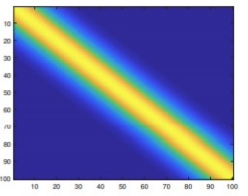
- $K$ is a banded diagonal matrix.
- The coefficient vector is $\alpha_n=[(K+\lambda I)^{-1}y]_n$
- Using the RBF, the predicted value is given by
- Pictorially, the predicted function $g_\theta$ can be viewed as the linear combination of the Gaussian kernels.
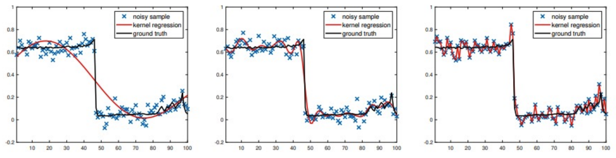
Effect of $\sigma$
- Large $\sigma$: Flat kernel. Over-smoothing
- Small $\sigma$: Narrow kernel. Under-smoothing
- Below shows an example of the fitting and the kernel matrix $K$.
Any Improvement?
- We can improve the above kernel by considering $x^n=[y_n, t_n]^\top$
- Define the kernel as
- This new kernel is adaptive (edge-aware).
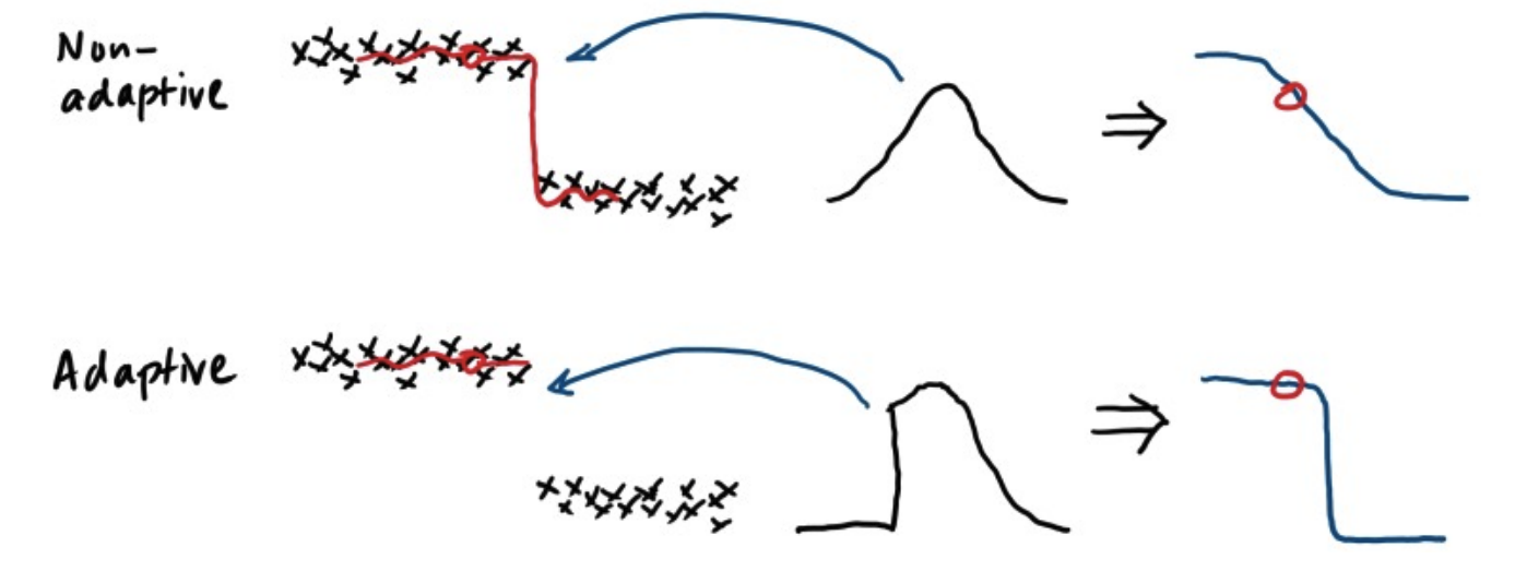
- This idea is known as bilateral filter in the computer vision literature.
- Can be further extended to 2D image where $x^n=[y_n, s_n]$, for some spatial coordinate $s_n$.
Kernel Methods in Classification
- The concept of lifting the data to higher dimension is useful for classification.
Kernels in Support Vector Machines
Example. RBF for SVM
- Radial Basis Function is often used in support vector machine.
- Poor choice of parameter can lead to low training loss, but with the risk of over-fit.
- Under-fitted data can sometimes give better generalization.